2.1 LEVELS OF ANALYSIS AND LOCATION UNITS

Later in this book we shall come to grips with some major questions of locational and regional macroeconomics; our concern will be with such large and complex entities as neighborhoods, occupational labor groups, cities, industries, and regions. We begin here, however, on a microeconomic level by examining the behavior of the individual components that make up those larger groups. These individual units will be referred to as location units.

Just how microscopic a view one takes is a matter of choice. Within the economic system there are major producing sectors, such as manufacturing; within the manufacturing sector are various industries. An industry includes many firms; a firm may operate many different plants, warehouses, and other establishments. Within a manufacturing establishment there may be several buildings located in some more or less rational relation to one another. Various departments may occupy locations within one building; within one department there is a location pattern of individual operations and pieces of equipment, such as punch presses, desks, or wastebaskets.

At each of the levels indicated, the spatial disposition of the units in question must be considered: industries, plants, buildings, departments, wastebaskets, or whatever. Although determinations of actual or desirable locations at different levels share some elements,¹ there are substantial differences in the principles involved and the methods used. Thus, it is necessary to specify the level to which one is referring.

We shall start with a microscopic but not ultramicroscopic view, ignoring for the most part (despite their enticements in the way of immediacy, practicality, and amenability to some highly sophisticated lines of spatial analysis) such issues as the disposition of departments or equipment within a business establishment or ski lifts on a mountainside or electric outlets in a house. Our smallest location units will be defined at the level of the individual dwelling unit, the farm, the factory, the store, or other business establishment, and so on. These units are of three broad types: residential, business, and public. Some location units can make independent choices and are their own "decision units"; others (such as branch offices or chain store outlets) are located by external decision.

Many individual persons represent separate residential units by virtue of their status as self-supporting unmarried adults; but a considerably larger number do not. In the United States in 1980, only about one person in twelve lived alone. About 44 percent of the population were living in couples (mostly married); nearly 30 percent were dependent children under eighteen; and a substantial fraction of the remainder were aged, invalid, or otherwise dependent members of family households, or were locationally constrained as members of the armed forces, inmates of institutions, members of monastic orders, and so on. For these types of people, the residential location unit is a group of persons.

In the business world, the firm is the unit that makes locational decisions (the location decision unit), but the "establishment" (plant, store, bank branch, motel, theater, warehouse, and the like) is the unit that is located. Further, the great majority of such establishments are the only ones that their firms operate. In general, a business location unit defined in this way has a specific site; but in some cases, the unit's actual operations can cover a considerable and even a fluctuating area. Thus, construction and service businesses have fixed headquarters, but their workers range sometimes far afield in the course of their duties; and the "location" of a transportation company is a network of routes rather than a point.

Nonprofit, institutional, social, and public-service units likewise have to be located. Though the decision may be made by a person or office in charge of units in many locations, the relevant locational unit for our purposes is the smallest one that can be considered by itself: for example, a church, a branch post office, a college campus, a police station, a municipal garage, or a fraternity house.

2.2 OBJECTIVES AND PROCEDURES FOR LOCATION CHOICE

Let us now take a locational unit—a single-establishment business firm, as a starting point—and inquire into its location preferences. First, what constitutes a "good" location? Subject to some important qualifications to be noted later, we can specify profits, in the sense of rate of return on the owners' investment of their capital and effort, as a measure of desirability of alternative sites. We must recognize, however, that this signifies not just next week's profits but the expected return over a considerable future period, since a location choice represents a commitment to a site with costs and risks involved in every change of location. Thus, the prospective growth and dependability of returns are always relevant aspects of the evaluation.

Because it costs something to move or even to consider moving, business locations display a good deal of inertia—even if some other location promises a higher return, the apparent advantage may disappear as soon as the relocation costs are considered. Actual decisions to adopt a new location, then, are likely to occur mainly at certain junctures in the life of a firm. One such juncture is, of course, birth—when the initial location must be determined. But at some later time, the growth of a business may call for a major expansion of capacity, or a new process or line of output may be introduced, or there may be a major shift in the location of customers or suppliers, or a major change in transport rates. The important point is that a change in location is rarely just that; it is normally associated with a change in scale of operations, production processes, composition of output, markets, sources of supply, transport requirements, or perhaps a combination of many such changes.²

It is quite clear that making even a reasonably adequate evaluation of the relative advantages of all possible alternative locations is a task beyond the resources of most small and medium-sized business firms. Such an evaluation is undertaken, as a rule, only under severe pressure of circumstances (a strong presumption that something is wrong with the present location), and various shortcuts and external aids are used. Perhaps the closest approach to continuous scientific appraisal of site advantages is to be found in some of the large retail chains. Profit margins are thin and competition intense; the financial and research resources of the firm are very large relative to the size of the individual store; and the stores themselves are relatively standardized, built on leased land, and easy to move. All these conditions favor a continuous close scrutiny of new site opportunities and the application of sophisticated techniques to evaluate locations.

Still more elaborate analysis is used as a basis for new location or relocation decisions by large corporations operating giant establishments, such as steel mills. These decisions, however, are few and far between, and involve in general a whole series of reallocations and adjustments of activities at other facilities of the same firm.

Within the limitations mentioned above we might characterize business firms as searching for the "best" locations for their establishments. This calls for comparison of the prospective revenues and costs at different locations.

What has been said about the choice of location for the business establishment will also apply in essence to many kinds of public facilities. Thus a municipal bus system will (or, one might argue, should) locate its bus garages on very much the same basis as would private bus systems. Since the system's revenues do not depend on the location of the garages, the problem is essentially that of minimizing the costs of building and maintaining the garages, storing and servicing the buses, and getting them to and from their routes.

The correspondence between public and private decisions is less close where the product is not marketed with an eye toward profit but is provided as a "public good" and paid for out of taxes or voluntary contributions. Thus an evaluation of the desirability of alternative locations for a new police station or public health clinic would have to include a reckoning of costs; but on the returns side, difficult estimates of quality and adequacy of service rendered to the community may be required. Where public authorities make the decision, the most readily available measuring rod might well be political rather than economic: Which location will find favor with the largest number of voters at the next election? This is in fact an essential feature of a democratic society.

Still more unlike the business firm example is that of the location of, say, a church or a nursing home. In neither case is success likely to be measured primarily in terms of numbers of people served or cost per person. Perhaps the judgment rests primarily on whether the facility is so located as to concentrate its beneficent effect on the particular neighborhood or group most needing or desiring it.

Finally, suppose we are considering the residence location of a family. Here again, cost is an important element in the relative desirability of locations. This cost will include acquiring or renting the house and lot, plus maintenance and utilities expenses, plus taxes, plus costs of access to work, shopping, school, social, and other trip destinations of members of the family. The returns may be measured partly in money terms, if different sites imply different sets of job opportunities; but in any event there will be a large element of "amenity" reflecting the family's evaluation of houses, lots, and neighborhoods; and this factor will be difficult to measure in any way.

There is a basic similarity in the location decision process of each of these cases: The definition of benefits or costs may differ in substance, but the goal of seeking to increase net benefit by a choice among alternative locations is common to all.

Further, it is important to note that a family, a business establishment, or any other locational unit is likely to be ripe for change in location only at certain junctures. There is ample and interesting evidence in Census reports that most changes of residence are associated with entry into the labor force, marriage, arrival of the first child, entry of the first child into school, last child leaving the household, widowhood, and retirement—though for specific families or individuals a move can also be triggered by a raise in salary, a new job opportunity, or an urban redevelopment project or other sudden change in the characteristics of a neighborhood.

For all types of locational units, locational choices normally represent a substantial long-range commitment, since there are costs and inconveniences associated with any shift. This commitment has to be made in the face of uncertainty about the actual advantages involved in a location, and especially about possible future changes in relative advantage. Homebuyers cannot foresee with any certainty how the character of their chosen neighborhood (in terms of access, income level, ethnic mix, prestige, tax rates, or public services) will change—though they can be sure it will change. The business firm cannot be sure about how a location may be affected in the future by such things as shifting markets or sources of supply, transportation costs and services, congestion, changes in taxes and public services, or the location of competitors.

Such uncertainties, along with the monetary and psychic costs of relocation, introduce a strong element of inertia. They also enhance the preferences for relatively "safe" locations such as "established" residential neighborhoods, business centers, or industrial areas. For business firms, the conservative tendency is reinforced by the fact that in a large corporate organization, decisions are made by managers whose earnings and promotion do not depend directly on the rate of profit made by the corporation so much as on maintenance of a satisfactory and stable earnings level and growth of output and sales. It is increasingly recognized that "profit maximization" may be an oversimplified conception of the motivating force behind business decisions, including those involving location.³

The effect of uncertainty from these various sources is to encourage spatial concentration of activities and homogeneity within areas. We should also expect a more sluggish response to change than would prevail in the absence of costs and uncertainties of locational choice. Further, if the firm is content with any of a number of "satisfactory" locations rather than insisting on finding the very best, there is substantial room for factors other than narrowly defined and measurable economic interests of the firm to enter the process of locational choice in an important way.

It is for this reason that the personal preferences of individual decision-makers are present even in the hard-nosed and impersonal corporation. Statistical inquiries into the avowed reasons for business location consistently report, however, that "personal considerations" figure most conspicuously in small, new, and single-establishment firms. Such considerations are least often cited in explaining locations of branch plants by large concerns (this being of course the case in which decision makers themselves are least likely to have a substantial personal stake in the matter, since they themselves will probably not have to live at the chosen location).

It would be wrong to label all personal elements of choice as irrational or as necessarily contributing to waste and inefficiency. The preference to locate one's job and one's home in a pleasant climate, a congenial community, and with convenient access to urban and cultural amenities may be hard to measure in dollars, but it is at least as real and sensible as one's preference for a higher money income. In the discussion of location factors that follows, the "inputs" and "outputs" should be understood to include even the less measurable and less tangible ones entailed in what are sometimes called nonbusiness motivations.

2.3 LOCATION FACTORS

Despite the great variety of types of location units, all are sensitive in some degree to certain fundamental location factors. That is to say, the advantages of locations can be categorized (for any type of unit) into a standard set of a few elements.

2.3.1 Local Inputs and Outputs

One such element of relative advantage is the supply (availability, price, and quality) of local or nontransferable⁴ inputs. Local inputs are materials, supplies, or services that are present at a location and could not feasibly be brought in from elsewhere. The use of land is such an input, regardless of whether land is needed just as standing room or whether it also contains minerals or other constituents actually used in the process, as in "extractive" activities such as agriculture or mining. Climate and the quality of the local water and air fall into the same category, as do topography and physical soil structure insofar as they affect construction costs, amenity, and convenience. Locally provided public services such as police and fire protection also are local inputs. Labor (in the short run at least) is another, usually accounting for a major portion of the total input costs. Finally, there is a complex of local amenity features, such as the aesthetic or cultural level of the neighborhood or community that plays an especially important role in residential location preferences. The common feature of all these local input factors is that what any given location offers depends on conditions at that location alone and does not involve transfer of the input from any other location.

In addition to requiring some local inputs, the unit choosing a location may be producing some outputs that by their nature have to be disposed of locally. These are called nontransferable outputs. Thus, the labor output of a household is ordinarily used either at home or in the local labor market area, delimited by the feasible commuting range. Community or neighborhood service establishments (barber shops, churches, movie theaters, parking lots, and the like) depend almost exclusively on the immediately proximate market; and, in varying degree, so do newspapers, retail stores, and schools.

One type of locally disposed output generated by almost every economic activity is waste. At present, only radioactive or other highly dangerous or toxic waste products are commonly transported any great distance for disposal; though the disposal problem is increasing so rapidly in many areas that we may see a good deal more long-distance transportation of refuse within our lifetimes. Other wastes are just dumped into the air or water or on the ground, with or without incineration or other conversion. In economic terms, a waste output is best regarded as a locally disposed product with negative value. The negative value is particularly large in areas where considerations of land scarcity, air and water pollution, and amenity make disposal costs high; this gives such locations an element of disadvantage for any waste-generating kind of unit.

It is not always possible to distinguish unequivocally between a local input and a local output factor. For example, along the Mahoning River in northeastern Ohio, the use of water by industries long ago so heated the river that it could no longer furnish a good year-round supply of water for the cooling required by steam electric generating stations and iron and steel works. In this instance, excess heat is the waste product involved. The thermal pollution handicap to heavy-industry development could be assessed either as a relatively poor supply of a needed local input (cold water) or as a high cost for disposing of a local output (excess heat). This is just one example of numerous cases in which a single situation can be described in alternative ways.

An often-neglected responsibility of government is to see that the costs of environmental pollution are imposed upon the polluting activity. The price of goods should reflect fully the social costs associated with consuming and producing them, if we value a clean environment. It is important to note that this guiding principle can be defended not only on the basis of equity but even more importantly on the basis of efficiency.

2.3.2 Transferable Inputs and Outputs

A quite different group of location factors can be described in terms of the supply of transferable inputs—such as fuels, materials, some kinds of services, or information—which can be moved to a given location from wherever they are produced. Here the advantage of a location depends essentially on its access to sources of supply. Some kinds of activities (for example, automobile assembly plants or department stores) use an enormous variety of transferred inputs from different sources.

Analogously, where transferable outputs are produced, there is the location factor of access to places where such outputs are in demand. The seller can sell more easily or at a better net realized price when located closer to markets.

2.3.3 Classification of Location Factors

To sum up, the relative desirability of a location depends on four types of location factors:

1. Local input: the supply of nontransferable inputs at the location in question
2. Local demand.' the sales of nontransferable outputs at the location in question
3. Transferred input: the supply of transferable inputs brought from outside sources to the location in question, reflecting in part the transfer cost from those sources

4. Outside demand: the sales of transferable outputs to outside markets; in particular, the net receipts from such sales, reflecting in part the transfer costs to those markets

It should be kept in mind that, throughout this chapter, "demand for output" means the demand for the output of the specific individual plant, factory, household, or other unit under consideration, and not the aggregate demand for all output of that kind. The demand for an individual unit's product at any given market is affected, of course, by the degree of competition; other things being equal, each unit will generally prefer to locate away from competitors. The same holds true for supply of an input. This and other interactions among competing units and the resulting patterns of location for types of activities are, however, the concerns of Chapters 4 and 5.

2.3.4 The Relative Importance of Location Factors

The classification of location factors just suggested is based on the characteristics of locations. But in order to rate the relative merits of alternative locations for a specific kind of business establishment, household, or public facility, one needs to know something about the characteristics of that kind of activity. Just how much weight should a pool hall or shoe factory or shipyard or city hall assign to the various relevant location factors of input supply and output demand?

There have been countless efforts to answer this question with respect to more or less specific classes of activities. Those concerned with location choice want to know the answer in order to pick a superior location. Those interested in community promotion seek the answer in order to make their community appear more desirable to industries, government administrators, and prospective residents.

Perhaps the commonest method of measurement is the most direct method: Ask the people who are making the locational decision. In many questionnaire surveys addressed to businessmen in connection with "industry studies," firms have been given a list of location factors, including such items as labor cost, taxes, water supply, access to markets, and power cost, and have been asked to rate them in relative importance, either by adjectives ("extremely important," "not very important," and so forth) or on some kind of simple point system.

This primitive approach is unlikely to provide any insights that were not already available and may sometimes be positively misleading. In the first place, it provides no real basis for a quantitative evaluation of advantages and disadvantages. If, for example, "taxes" are given an importance rating of 4 by some respondent, and "labor costs" a rating of 2, we still do not know whether a tax differential of 3 mills per dollar of assessed property valuation would offset a wage differential of 10 cents per man-hour. The respondent probably could have told us after a few minutes of figuring, but the question was not put to him or her in that way. A further shortcoming of the subjective rating method is that respondents are implicitly encouraged to overrate the importance of any location factors that may arouse their emotions or political slant, or if they feel that their response might have some favorable propaganda impact. It has been suggested, for example, that employers have often rated the tax factor more strongly in subjective-response surveys than would be supported by their actual locational choices.

A more quantitative approach is often applied to the estimation of the strength of various location factors involving transferred inputs and output. For example, we might seek to determine whether a blast furnace is more strongly attracted toward coal mines or toward iron ore mines by comparing the total amounts spent on coal and on iron ore by a representative blast furnace in the course of a year, and such a figure is easily obtained. Unfortunately, this method could not be relied on to give a useful answer where the amounts are of similar orders of magnitude. We might use it to predict that a blast furnace would be more strongly attracted to either coal mines or iron ore mines than it would be to, say, the sources of supply of the lubricating oil for its machinery; but it may be assumed that we know that much without any special investigation. A little closer to the mark, perhaps, would be a comparison between the annual freight bills for bringing coal to blast furnaces⁵ and for bringing iron ore to those furnaces. But this comparison is obviously influenced by the different average distances involved for the two materials as well as by the relative quantities transported, so again it tells us little.

We might instead simply compare tonnages and say that if it takes coke from two tons of coal to smelt one ton of iron ore, the choice of location for a blast furnace should weight nearness to coal mines twice as heavily as nearness to iron ore mines. Here we are getting closer to a really informative assessment (for these two location factors alone), although our answer would be biased if one of the two inputs travels at a higher transport cost per ton-mile than the other (a consideration to be discussed later in this chapter).

It would appear that in order to assess the relative importance of various location factors for a specific kind of activity we need to know the relative quantities of its various inputs and outputs. If, for example, we want to know whether labor cost is a more potent location factor than the cost of electric power, we first need to know how many kilowatt-hours are required per man-hour. If this ratio is, say, 20, and if wages are 10 cents an hour higher in Greenville than in Brownsville, it would be worthwhile to pay up to ½ cent more per kilowatt-hour for power in Brownsville (assuming of course that these two locations are equal with respect to all other factors, including labor productivity).

This kind of answer is what the locator of a plant would need; but it should be noted that it is not necessarily indicative of the degree to which we should expect to find this kind of activity attracted to cheap power as against cheap labor locations. Perhaps differentials of ½ cent per kilowatt-hour or more are frequently encountered among alternative locations for this industry, whereas wage differentials of as much as 10 cents an hour are rather rare for the kind of labor it uses. In such a case, the power cost differentials would show up more prominently as decisive locational determinants than would wage differentials. Thus we conclude that, for some purposes at least, we need to know something about the degree of spatial variability of the input prices corresponding to the location factors being weighed against one another.

When we consider a location factor such as taxes, we encounter a further complication: There is no appropriate way to measure the quantity of public services that a business establishment or household is buying with its taxes or to establish a "unit price" for these services. The only way in which we can get a measure of locational sensitivity to tax rates is to refer to the actual range of rates at some set of alternative locations and translate these into estimates of what the tax bill per year or per unit of output would amount to at each location. This procedure has been followed in some actual industry studies, such as the one carried out by Alan K. Campbell for the New York Metropolitan Region Study.⁶ A major relevant problem is how to measure and allow for any differences in the quality of public services; this is related to tax burdens, although not in the close positive correspondence that one might be tempted to assume.

Insight into still another problem of assessing relative strength of location factors comes from consideration of the implications of a differential in labor productivity. If wages are 10 percent higher in Harkinsville than in Parkston, but the workers in Harkinsville work 10 percent faster, the labor cost per unit of output will be the same in both places, and one might infer that neither place will have a net cost advantage over the other. In fact, however, the speedier Harkinsville workers will need roughly 10 percent less equipment, space, and the like than their slower counterparts in Parkston to turn out any given volume of output; so there will be quite a sizable saving in overhead costs in Harkinsville. This advantage, though resulting from a quality difference in production workers, will appear in cost accounts under the headings of investment amortization costs, plant heating and services, and perhaps also payroll of administrative personnel and other nonproduction workers.

A somewhat different kind of identification problem arises when there are substantial economies or diseconomies of scale. Suppose we are trying to compare two locations for the Ajax Foundry, with respect to supply of the scrap metal it uses as a principal input. The going price of scrap metal is lower in Burton City than in Evansville; but only relatively small amounts are available at the lower price. If Ajax were to operate on a large scale in Burton City, it would have to bid higher to attract scrap from a wider supply area, whereas in Evansville scrap is generated in much larger volume and supply would be very elastic: Ajax's entry as a buyer would not drive the price up appreciably. In this case, Ajax must decide whether the economies of larger volume would be sufficient to make Evansville the better location or so slight that it would be better to operate on a reduced scale in Burton City. Similarly, some locations will offer a more elastic demand for the output than others, and here again the choice of location will depend in part on economies of scale.

The foregoing discussion has brought to light some of the less obvious complexities of the problem of measuring the relative importance of the various factors affecting the choice of location for a specific business establishment or other unit. It should now be clear that definite quantitative "weights" can be assigned to the various factors only in certain cases (to be discussed later in this chapter) involving transfer cost. It has also been argued that the relative influence of the various factors upon location depends on the amounts and kinds of inputs and outputs and on the geographical patterns of variation of the respective input supplies and output demands.

2.4 SPATIAL PATTERNS OF DIFFERENTIAL ADVANTAGE IN SPECIFIC LOCATION FACTORS

If one views the earth's surface from space, it looks completely smooth—after all, the highest mountain peaks rise above sea level by only about 1/13 of 1 percent of the planet's radius. A closer view makes many parts of the earth's surface look very rough indeed. Again, if one looks at a table-top, it appears smooth, but a microscope will disclose mountainous irregularities.

The same principle applies to spatial differentials in a location factor: The interregional (macrogeographic) pattern is quite different from the local (microgeographic) pattern. For example, we should not expect land cost to be relevant in choosing whether to locate in Ohio or in Minnesota; but if the choice is narrowed down to alternative sites within a particular metropolitan area, land cost will indeed be important. Large differences may appear even within one city block.

Labor supply and climate, in contrast, are examples of location factors where there is little microgeographic variation (say, within a single county or metropolitan area), but wide differences prevail on a macrogeographic scale involving different regions.

Locational alternatives and choices are generally posed in terms of some specific level of spatial disaggregation. The choice is among sites in a neighborhood, among neighborhoods in an urban area, among urban areas, among regions, or among countries. No useful statements about location factors, preferences, or patterns can be made until we first specify the level of comparison or the "grain" of the pattern we are concerned with.

This principle was in fact implicit in our earlier distinction between local and transferable inputs and outputs. After all, the only really non-transferable inputs are natural resources or land, including topography and climate. In a very fine-grained comparison of locational advantages (say, the selection of a site for a residence or retail store within a neighborhood), we must recognize that all other inputs and all outputs are really transferred, though perhaps only for short distances. Water, electric energy, trash, and sewage all require transfer to or from the specific site. Selling one's labor or acquiring schooling requires travel to the work place or school; selling goods at a retail store requires travel by customers.

Accordingly, our distinction between local and transferable inputs is a flexible one: It will vary according to how microgeographic or macrogeographic a view of location we are taking for the situation at hand. Thus if we are concerned with choices of location among cities, "local" means not transferable between cities. Some inputs or outputs properly regarded as local in such a context are properly regarded as transferable between sites or neighborhoods within a city.

What, then, are the possible kinds of spatial differential patterns for a location factor as among various locations at any prescribed level of geographic detail?

The simplest pattern, of course, is uniformity: All the locations being compared rate equally with respect to the location factor in question. For example, utility services are commonly provided at uniform rates over service areas far larger than neighborhoods, often encompassing whole cities or counties. Wage rates in an organized industry or occupation are generally uniform throughout the district of a particular union local, and in industries using national labor bargaining they may even be uniform all over the country. Tax rates are in general uniform over the whole jurisdiction of the governmental unit levying the tax (for example, city property taxes throughout a city, state taxes throughout a state, and national taxes nationwide). Many commodities are sold at a uniform delivered price over large areas or even over the whole country. Climate may be, for all practical purposes, the same over considerable areas.

The special term ubiquity is applied to inputs that are available in whatever quantity necessary at the same price at all locations under consideration. Air is a ubiquity, if we are indifferent about its quality. Federal tax stamps for tobacco or alcohol are a ubiquity over the entire country. If an input is ubiquitous, then its supply cannot be a location factor—being equally available everywhere, it has no influence on location preferences.

The demand-side counterpart of a ubiquity is of course an output for which there is the same demand (in the sense of equally good access to markets) at all locations under consideration. There does not seem to be any special technical term for this, and it is in fact a much rarer case than that of an input ubiquity. Perhaps we could illustrate it. Imagine some type of business that distributes its product by letter mail, but with speedy delivery not being a consideration. In such a case, proximity to customers is inconsequential; demand for the output is in effect ubiquitous. The reason, in this special case, is that the postal service makes no extra charge for additional miles of transportation of letters.

A different pattern of advantage for a location factor can be illustrated by market access for wheat growers. The demand for their wheat is perfectly elastic, and what they receive per bushel is the price set at a key market, such as Chicago, minus the handling and transportation Charges. The net price they receive will vary geographically along a rather smooth gradient reflecting distance from Chicago. The locational effect of the output demand factor can be envisaged as a continuous economic pull in the direction of Chicago. Similar pull effects reflecting access advantage operate within individual urbanized areas. For example, workers' residence preferences are affected by the factor of time and cost of commutation to places of employment.

Another kind of systematic pattern involves differential advantage according to the size of the town or city in which the unit is located. This might apply to certain location factors involving the supply of or the demand for inputs or outputs that are not transferable between cities. It would be surprising to find any kind of differential advantage that is precisely determined by size of place; but there are many location factors that in fact show roughly this kind of pattern. Some activities cater to local markets and cannot operate at a minimum efficient scale except in places of at least a certain minimum size. In selecting a location for such an activity, the first step in the selection process might well be to winnow down the alternatives to a limited set of sufficiently large places. Thus one would not ordinarily expect to find patent lawyers, opera houses, investment bankers, or major league baseball teams in towns or small cities.

Finally, there are location factors for which the spatial pattern of advantage is not obviously systematic at all—that is, it cannot be described or predicted in any reasonably simple terms, although it is not necessarily accidental or random. Tax rates, local water supply, labor supply, and quality of public services seem to fall into this category. Some general statements can be made to explain the broad outlines of the pattern (such a statement is attempted for labor costs in Chapter 10); but for making comparisons for actual selection of locations there is no way of avoiding the necessity of collecting information about every individual location that we wish to consider.

Among the kinds of patterns of differential advantage that location factors may assume, three in particular merit further discussion: those determined by transfer costs, those determined by size of city or local market, and those involving labor cost. We turn here to the transfer cost case, reserving the other two for consideration in later chapters.

2.5 TRANSFER ORIENTATION

Until fairly recently, location theory laid exaggerated emphasis on the role of transportation costs, for a number of reasons. Interest was particularly focused on interregional location of manufacturing industries, for which transportation costs are in fact relatively more important and obvious than for most other kinds of activities. Moreover, the effect of transfer costs on location is more amenable to quantitative analysis than are the effects of other factors, so that the development of a systematic body of location theory naturally tended to use transfer factors as a starting point and core. A basic rationale for emphasis on transfer advantages is given by Walter Isard: "Only the transport factor and other transfer factors whose costs are functionally related to distance impart regularity to the spatial setting of activities."⁷

We can speak of a particular activity as transfer-oriented⁸ if its location preferences are dominated by differential advantages of sites with respect to supply of transferable inputs, demand for transferable outputs, or both. Similarly, we can call an activity labor-oriented where the locational decisions are usually based on differentials in labor cost.

Let us look first at a simple model of transfer orientation. In order to facilitate the development of this model, it will be helpful to consider the concept of production. In traditional nonspatial economic theory, production is viewed as a transformation process. One uses factors of production in some combination in order to produce a good or service; thus, one "transforms" inputs into outputs. Later in this chapter, we shall find that the nature of that transformation process may itself influence the location decision. However, for our immediate purposes, it is important to recall from the discussion of transfer factors earlier in this chapter that the activity of a locational unit involves much more than transformation per se. It also involves the acquisition of inputs and the distribution of output, both of which may require transfer over substantial distances. The same might be said about the activity of a household or other nonprofit establishment. Space plays an essential role in economic activity.

Given this, it is easy to recognize that the costs incurred by the firm also have a spatial component. If we are to understand the behavior of business establishments, we must be concerned with the costs associated with bringing inputs together and distributing outputs, just as we are concerned with the costs of transforming inputs into output. The total costs, therefore, include these three components, and a locational unit that is seeking to minimize costs or maximize profits must take them all into consideration.

Let us focus now on the behavior of a single-establishment business firm aiming to maximize profits (revenue less cost) and seeking the best location for that purpose. We shall see that the problem can be quite complex, so it will be helpful to start off with some simplifying assumptions that can later be relaxed.

First, we shall assume that there are markets for this unit's output at several points, but that the unit is too small to have any effect on the selling price in any of those markets. In other words, demand for the unit's output is perfectly elastic, and it must take the prevailing prices as given, regardless of its volume of sales. The firm has to pay for the costs of delivering its output, so there is some incentive to locate at or near a market. Costs associated with distribution of output rise as distance from the market increases.

We simplify the case further by making exactly the same kind of assumption on the input side as we have just done on the output side. In other words, the kinds of transferable inputs our unit uses are available at different sources, but at each source the supply is perfectly elastic, so the price can be taken as given regardless of how much of the input is bought. Consequently, there will be a cost incentive for the unit to locate at or near a source of transferable inputs, in addition to the already mentioned incentive to locate at or near a market.

Our third assumption is that the unit's processing costs (using local inputs) will not vary with either location or scale of operations.

These three simplifying assumptions bypass some highly important factors bearing on the choice of locations, which will be addressed in later chapters. What we have done for the present is to reduce the problem of a maximum-profit location to the much simpler problem of minimizing transfer costs per unit of output, by postponing consideration of such factors as processing-cost differentials, economies or diseconomies of scale, and control over buying or selling prices by the business unit under consideration.

Finally, we can simplify the problem of minimizing transfer costs by letting transfer costs be uniform per ton mile, regardless of distance or direction. This assumption of what is called a uniform transfer surface postpones (until the next chapter) a recognition of the various differentials that typically appear in transfer costs in the real world.

If the unit in question uses only one kind of transferable input (say, wood) and produces one kind of transferable output (say, baseball bats), then the choice of the most profitable location is easy to describe. The first question to be settled is that of input orientation versus output orientation. Will it be preferable to make the bats at a wood source, or at the market, or at some point on the route between source and market? There are no other rational possibilities, since a detour would obviously be wasteful.

The question can be settled by considering any pair of source and market locations, as in Figure 2-1. The possible locations are the points on the line SM. Input costs are reduced as the point is shifted toward S, but receipts per unit output are increased as the location is shifted the other way, toward M; that is, transport costs associated with the delivery of the final product are reduced with movements toward the market. Which attraction will be stronger? There is a close physical analogy here to a tug of war between two opposing pulls, but how are their relative strengths measured? Let the relative weights of transferred input and transferred output be w_m and w_q respectively (i.e., let it take w_m tons of the material to make w_q, tons of the product). The material travels at a transfer cost of r_m per ton-mile and the product at r_q per ton-mile. Moving the processing location a mile closer to the market M and thus a mile farther from the material source S will save w_q,r_q, in delivery cost but will add w_mr_m to the cost of bringing in the material. The w_q,r_q, and w_mr_m are called the ideal weights of product and material respectively, since they measure the strengths of the opposing pulls in the locational tug of war between material source and market, and take account of both the relative physical weights and the relative transfer rates on material and product. Production will ideally take place at the market or at the material source, depending on which of the ideal weights is the greater.

A numerical example may help to clarify this point. Let us say that, in the course of a typical operating day, 2000 tons of the transferable input are required and that the transferable output weighs 250 tons. Further, assume that the transfer rate on this input is 2 cents per ton-mile, whereas the transfer rate on the output is 32 cents per ton-mile. Given these conditions, delivery costs on the output would decrease by $80 (250 × 32¢) per day for every mile that the location is shifted toward the market and away from the material source. However, transfer costs on the input would increase by only $40 (2000 × 2¢) per day for each such move. We might express these ideal weights in relative terms as $80/$40 or 2/1 in favor of the transferable output, and in this example the locational unit would be drawn toward the market.

It is of course conceivable that the two ideal weights might be exactly equal, suggesting an indeterminate location anywhere along the line SM. This special case would appear, however, to be about as likely as flipping a coin and having it stand on edge. Indeed, certain further considerations to be introduced in the next chapter make such an outcome even more improbable. So it is a good rule of thumb that if there is just one market and just one material source, transfer costs can be minimized by locating the processing unit at one of those two points and not at any intermediate point.

We can establish a rough but useful classification of transfer-oriented activities as input-oriented (characteristically locating at-a transferable-material source) and output-oriented (characteristically locating at a market). Various familiar attributes of activities play a key role in determining which orientation will prevail.

For example, some processes are literally weight-losing: Part of the transferred material is removed and discarded during processing so that the product weighs less. In such physically weight-losing processes, clearly a location at the material source gets rid of surplus weight before transfer begins, reduces the total weight transferred, and thus will be preferred unless the shipping rate on the product exceeds that on the material sufficiently to compensate for the reduction in total ton-miles.

The opposite case (gain of physical weight in the course of processing) can occur when some local input such as water is incorporated into the product, thus making the transferred output heavier than the product. Here (in the absence of a compensating transfer rate differential) the preferred location will be at the market, because it pays to introduce the added weight as late as possible in the journey from S to M.

Both of the above two cases entail, essentially, differences in the physical weight component of the ideal weights. But as the further illustrative cases in Table 2-1 show, the transfer orientation of an activity can be based on some characteristic and logical differential between the transfer rate on the output and the transfer rate on the input. This can occur when the production process is associated with major changes in such attributes as bulk, fragility, perishability, or hazard.

*In some of these cases, the actual orientation reflects a combination of two or more of the listed process characteristics. Thus some kinds of canning and preserving involve important weight and bulk loss as well as reduction of perishability. A further reason for the usual output orientation of modern by-product coke ovens is that the bulkiest output, gas, is in demand at the steelworks where the coking is done. Coke produced by the earlier "beehive" process was generally made at coal mines, since weight loss more than offset fragility gain. (The gas went to waste.)

Processing activities of course usually result in a product more valuable than the required amount of transferred inputs; and for a number of good reasons, transfer rates tend to be higher on more valuable commodities. Risk of damage or pilferage is greater; there is a greater interest cost on the working capital tied up in the commodity in transit; and (as will be explained in the next chapter) transfer agencies commonly have both the incentive and the opportunity to discriminate against high-value goods in setting their tariffs. Value gain in processing is thus an activity characteristic favoring market orientation.⁹

An important observation of ideal weights is that they are real and measurable even when physical weight is zero or irrelevant. We can directly evaluate the ideal weights of inputs or outputs such as electric energy, communications, and services by determining the costs of transferring them an additional mile and then comparing this information with the cost of an additional mile of transfer on the appropriate corresponding quantity of whatever other transferable input or output is involved in the process.

As mentioned earlier, the comparison of ideal weights permits at least tentative categorizations of transfer-oriented activities as input-oriented or output-oriented and points the way toward more specific determination of locational preference for specific units and activities. Suppose for example that we have determined that the unit we are considering is output-oriented. Then the choice of possible locations is immediately narrowed down to the set of market locations, and all that remains is to select the most profitable of these.

For each market location, there will be one best input source, which can supply the transferred input to that market more cheaply than can any other source. Figure 2-2 pictures this pairing of sources and markets. The profitability of location at each market can thus be calculated, and a comparison of these profitabilities indicates where the unit should locate.

The situation shown in Figure 2-2 has some other features to be noted. First, the best input source for a location at any given market is not necessarily the nearest. A more remote low-cost source may be able to deliver the input more cheaply than the higher-cost source that is closer at hand. Second, any one input source may be the best source for more than one market location (but not conversely). Third, there may be some input sources that would not be used by any of the market locations. Finally, Figure 2-2 could be used to picture the ease of an input-oriented unit, by simply interchanging the Ss and Ms. If the unit is input-oriented to a single kind of input, all that is needed is to choose the best source at which to locate, and then there will be a best market to serve from that location.

Next, let us complicate matters a little by considering an activity that uses more than one kind of transferable input (for example, a foundry that uses fuel and metals plus various less important inputs such as wood for patterns and sand for molds). Initially we shall assume that the various inputs are required in fixed proportion.

We now have three or more ideal weights to compare. For each ton of output, there will be required, say, x tons of one transferable input plus y tons of another. The question of orientation is now somewhat more complex. In Figure 2-3, which pictures one market and one source for each of two kinds of input, the most profitable location may be at any one of those three points or at some intermediate point. Retaining our assumption of a uniform transfer surface, we can see immediately that the choice of intermediate locations is restricted to those inside or on the boundaries of the triangle formed by joining the input sources and market points.

This constraint upon possible locations will always apply when there are just three points involved, as in Figure 2-3. If there are more market or source points, so that we have a locational polygon of more than three sides, the constraint will still apply if the polygon is "convex" (that is, if none of its corners points inward).

Looking at Figure 2-3, we can envisage three ideal weights as forces influencing the processing location, each attracting it toward one of the corners of the triangle. The most profitable location is where the three pulls balance, so that a shift in any direction would increase total transfer costs.¹⁰

In the case of three or more factors of transfer orientation, we can no longer be positive about which force will prevail. In fact, we can really be sure only if one of the ideal weights involved is predominant: that is, at least equal to the sum of all the other weights.

It does not follow, however, that an intermediate location will be optimal in all cases in which no single ideal weight predominates. The outcome in such a case depends on the shape of the locational figure: that is, the configuration of the various source and market points in space. For example, in Figure 2-4 the configuration is such that the activity would be input-oriented to source S₂ even if the relative weights were 3 for S₁, 2 for S₂ and 4 for the market M.¹¹ But with the same weights and a figure shaped like that in Figure 2-3, an intermediate location within the triangle would be optimal, and we could not describe the activity as being either input-oriented or output-oriented.

We find, then, that it is not as easy as it first appeared to characterize by a simple rule the orientation of any given type of economic activity. If the activity uses more than one kind of transferable input (and/or if it produces more than one kind of transferable output), we may well find that an optimum location can sometimes be at a market, sometimes at an input source, and sometimes at an intermediate point. The steel industry is a good example of this. Some steel centers have been located at or near iron ore mines, others near coal deposits, others at major market concentrations, and still others at points not possessing ore or coal deposits or major markets but offering a strategic transfer location between sources and markets. Intermediate and varying orientations are most likely to be found in activities for which there are several transferable inputs and outputs of roughly similar ideal weight. In the next chapter, when we drop the simplifying assumption of a uniform transfer surface, it will be possible to gain some additional perspective on rules of thumb about transfer orientation.

2.6 LOCATION AND THE THEORY OF PRODUCTION

So far we have been assuming that for a particular economic activity the physical weights of transferred inputs and outputs were in fixed proportion; that is, the production recipe could not be altered. In practice, this is often not true. For example, in the steel industry, steel scrap and blast furnace iron are both used as metallic inputs, but it is possible to step up the proportion of scrap at times when scrap is cheap and to design furnaces to use larger proportions of scrap at locations where it is expected to be relatively cheap. In almost any manufacturing process, in fact, there is at least some leeway for responding to differences in relative cost of inputs and relative demand for outputs. The same principle also applies more broadly to nonmanufacturing activities, and it includes substitution among nontransferable as well as transferable inputs and outputs. Thus labor is likely to be more lavishly used where it is cheap, and to be replaced by labor-saving equipment where it is expensive.

In order to explore some of the implications associated with input substitutions of this sort, consider the locational triangle presented in Figure 2-5.¹² As in earlier examples, we shall once again consider the decision of a locational unit with two transferable inputs (x₁ located at S₁ and x₂ located at S₂) and one transferable output with a market located at M. To focus attention on the effects of input substitution, we shall take delivery costs as given by limiting our consideration to locations I and J, which are equidistant from the market, and we shall assume that the same production technology is applicable at either location. The arc IJ includes additional locations at that same distance from the market, which we shall consider later.

The delivered price of a transferable input is its price at the source plus transfer charges. In the present example, there are two such inputs, x₁ and x₂. Their delivered prices are respectively

where p₁ and p₂ are the prices of each input at is source, and r₁ and r₂ represent transfer rates per unit distance for these inputs. The distance from each source to a particular location such as I or J is given by d₁ and d₂.

It is significant that the relative prices of the two inputs will not be the same at I as at J. Location I is closer than J to the source of x₁, but farther away from the source of x₂. So in terms of delivered prices, x₁ is relatively cheaper at I and x₂ is relatively cheaper at J. The total outlay (TO) of the locational unit on transferable inputs is

This equation may be reexpressed as

For any given total outlay (TO), the possible combinations of the two inputs that could be bought are determined by equation (2), and these combinations can be plotted by equation (3) as an iso-outlay line.¹³

Locations I and J have different sets of delivered prices, and therefore the possible combinations of inputs x₁ and x₂that any given outlay TO can buy will vary according to location. Figure 2-6 presents the iso-outlay lines associated with locations I and J for a given total outlay and prices. The iso-outlay line associated with location I is represented by AA', and that associated with location J is represented by BB'. The shorter distance involved in transporting input 1 to I rather than to J implies that the price ratio (p'₂/p'₁) will be greater at location I. Since this price ratio determines the slope of the iso-outlay line (see equation (3) and footnote 13), we find that the slope of AA' is greater than that of BB'. Also, it is important to recognize that the slope of any ray from the origin, such as OR, defines a particular input ratio (x₁/x₂). Movement out along such a ray implies that more of each input is being used and that the rate of output must be increasing.

Because we have relaxed the assumption restricting the ratio in which transferable inputs are used, any ray could potentially identify the input proportion used by the locational unit. Notice, however, that if the firm chose to use the input ratio identified with OR', it could produce more output for any given total outlay by producing at location I and accepting the iso-outlay line AA'. In fact, for any input ratio (x₁/x₂) greater than that implied by OR, location I would be efficient in this sense. By implication, if the production decision is such that an input ratio greater than that implied by OR is used, the unit would locate at I. Similarly, for any input ratio less than OR, BB' would be efficient and the unit would locate at J. The effective iso-outlay line is, therefore, represented by ACB’.

The location decision and the production decision are therefore inextricably bound. As decisions are made concerning optimal input combination for a given level of output, the firm must at the same time consider its locational alternatives. The simultaneity of this process can be illustrated by reference to Figure 2-6. The line denoted by Q₀ in that figure is referred to as an isoquant, or equal product curve, and characterizes the unit's ability to substitute between inputs in the production process. It indicates that the rate of output Q₀ can be produced by every input combination represented by the coordinates of a point on that line. So for any specified output, there is a location and an input combination that will minimize the total cost of inputs. In our example, Q₀ can be produced most efficiently at the input ratio represented by OR" and this, in turn, implies location at J.¹⁴

We might characterize the outcome of the decision process in this example as a locational orientation towards the input x₂. The word "orientation'' is used in a somewhat less restrictive way here than in previous examples. Here, it is only meant to suggest that the outcome of the production-location decision is that the unit was drawn toward a location closer to x₂ as a result of the nature of its production process and the structure of transfer rates.

While the problem analyzed above concerns a decision between two locations, it can be extended to include all possible points within a locational triangle such as that presented in Figure 2-5. One might think of this generalization as proceeding in two steps. First, many points along an arc of fixed radius from the market (e.g., the arc IJ in Figure 2-5) can be considered, rather than simply concentrating on two such points. In this ease, even small changes in the ratio of delivered prices could alter the optimal input mix and the balance of ideal weights, forcing the firm to consider a new location in the long run.¹⁵ Second, the economic incentives drawing the location to points of varying distance from the market could be analyzed. Here again, consideration of ideal weights is in order, with the balance of opposing forces drawing the unit closer to the market or the material sources.

The nature of the production process can also affect location decisions as the scale of production increases or decreases. Changes in the rate of output may well imply changes in the optimal input mix, so that there will be changes in ideal weights and probably in locational preferences. Such a situation is depicted in Figure 2-7. For this particular production process, a change in the rate of output from Q₀ to Q₁ would imply a new equilibrium location; in the long run, a switch from location J to location I is indicated as the rate of output is increased. The reason for this is apparent if one recognizes that the optimal input ratio changes from that represented by OR" to that represented by OR'; hence, at the greater rate of output, larger amounts of x₁ are used relative to x₂ per unit of production. As the ideal weights change, a location closer to the source of x₁ is, therefore, encouraged.

It is possible also that increases in the scale of operations may imply less than proportionate increases in the requirements for one or more of the transferred inputs. Thus large-scale steel making may yield some savings in fuel requirements per ton of output. Operations that have this characteristic would be drawn toward the market, because the ideal weight of the inputs decreases relative to that of the final product with increases in the scale of production.

However, contrary forces may also be evidenced. Increases in scale may require the use of more transferable inputs and fewer local inputs per unit of output—for example, using more material and less labor. In this instance, the ideal weight of the final product may actually be reduced relative to the ideal weight of transferable inputs. Orientation would then be shifted away from the market.

Thus valid generalizations concerning the effect of the scale of production on location decisions are difficult to make.¹⁶ Indeed, at a practical level, changes in scale and changes in technology often go hand in hand, lessening the usefulness of analysis based on production processes currently employed. The essential point is that one must look to changes in ideal weights in order to assess changes in locational orientation. As relative prices or the scale of operations change over time, ideal weights may be affected.

2.7 SCALE ECONOMIES AND MULTIPLE MARKETS OR SOURCES

Another simplifying assumption that we applied in our discussion of transfer orientation was that a unit disposes of all its output at one market and obtains all its supply of each input from one source. This accords with reality in many, but by no means all, cases. If a seller's economies of scale lead it to produce an output that is substantial in relation to the total demand for that output at a single market, it will face a less than perfectly elastic demand in any one market and it may be profitable for it to sell in such additional markets as are accessible. In that event, the location factor of "access to market" will entail nearness not just to one point, but to a number of points or a market area. Similarly, it may find that it can get its supplies of any particular transferable input more cheaply by tapping more than one source if the supply at any one source is not perfectly elastic.

Figure 2-8 shows how we might, in principle, analyze the market-access advantages of a specific location in terms of possible sales to a number of different market points. In this illustration, there are five markets in all, assumed to be located at progressively greater distances from the seller. If the demand curve at each of those markets is identical in terms of quantities bought at any given delivered price (price of the goods delivered at the market), then the demand curves as seen by the seller (that is, in terms of quantities bought at any given level of net receipts after transfer costs are deducted) will be progressively lower for the more distant markets. This is shown by the series of five steeply sloping lines in the left-hand part of the figure. If we now add up the sales that can be made in all markets combined, for each level of net receipts, we obtain the aggregate demand curve pictured by the broken line ABCDEFG. For example, at a net received price of OH (after covering transfer costs) it is possible to sell HI, HJ, HK, HL, and HM in the five markets respectively. His total sales will be HF, which is the sum of HM plus MN (=HL) plus NP (=HK) plus PQ (=HJ) plus QF (=HI).

This aggregate demand schedule and the costs of operating at the location in question will determine what profits can be made there by choosing the optimum price and output level,¹⁷ At possible alternative locations, both market and cost conditions will presumably be different, giving rise to spatial differentials in profit possibilities.

Although the foregoing may describe fairly well what determines the likelihood of success at a given location, it is hardly a realistic description of the kind of analysis that underlies most location decisions. Following are descriptions of some cruder procedures for gauging access advantage of locations in the absence of comprehensive data.

2.8 SOME OPERATIONAL SHORTCUTS

For simplicity's sake, let us consider just the question of evaluating access to multiple markets. If, for example, a market-oriented producer seeks the best location from which to serve markets in fifty major cities in the United States, how might it proceed?

What it wants is some sort of "geographical center" of the set of fifty markets. Suppose that this center were to be defined as a median point so located that half of the aggregate market lay to the north and half to the south of it, and likewise half to the east and half to the west¹⁸ Then (if it were to be assumed that transport occurs only on a rectilinear grid of routes) the producer would have the location from which the total ton-miles of transport entailed in serving all markets would be a minimum. This is an application of the principle of median location.

Naturally, a number of objections might be made to this procedure. One of the most obvious is that it is illogical to assume that our producer's sales pattern is independent of its location. It would be more reasonable to assume that the producer would have a smaller share of the total sales in markets more remote from its location, reflecting higher transport charges and other aspects of competitive disadvantage.

One way to get around this difficulty would be to decide that the producer is really primarily interested in market possibilities only within, say, a radius of 400 miles, or only within the range of overnight truck delivery. It could then demarcate such areas around various points and select as its location the center of the area having the largest market volume.

A somewhat more sophisticated procedure would be to apply a systematic distance discount in the evaluation of markets by calculating what is called an index of market access potential for each of a number of possible locations. Thus to compute the potential index Pi for any specific production location (i), the producer would divide the sales volume of each market (j) by the distance D_ij from (i) to (j) and then add up all the resulting quotients. Such potential measures have been widely used, with the distance (or transport costs, if ascertainable) commonly raised to some power such as the square. If the square of the distance is used, the potential formula becomes

(where M is market size and D is distance); and any given market has the same effect on the index as a market four times as big but twice as far away. In any ease, when the potential index P has been calculated for various possible locations, the location having the largest P can then be rated best with respect to access to the particular set of markets involved.

This measure of "potential," in which each source of attraction has its value "discounted for distance," is also generically known as a gravity formula or model—particularly when the attractive value is deflated by the square of distance over which the attraction operates. The reference to gravity reflects analogy to Newton's law of gravitation (bodies attract one another in proportion to their masses and inversely in proportion to the square of the distance between them). William J. Reilly in 1929 proclaimed the Law of Retail Gravitation on the basis of an observed rough conformity to this principle in the case of retail trading areas (a subject to be examined in more detail in Chapter 8), and John Q. Stewart and a host of others subsequently discovered gravity-type relationships in a wide variety of economic and social distributions. Gravity and potential measures have in fact been applied to almost every important measurable type of human interaction involving distance, and numerous variants of the basic formula have been devised, some of which we shall have occasion to examine later.¹⁹ All the shortcut methods described here have been widely used. Though they have been explained here in terms of the measurement of access to markets, or output access of potential locations, they are equally applicable to assessment of the input access potential of locations, when a unit is drawing on more than one source of the same transferable input. The measures can apply also to cases involving the transfer of services rather than goods—for example, measuring the job-access potential of various residence locations where a choice of job opportunities is desirable, or measuring the labor-supply access potential of alternative locations for an employer.

But at best, when a unit can serve many markets and/or draw from many input sources, the appraisal of alternative locations in terms of access is a complex matter. There is likely to be little opportunity to use the simple devices discussed earlier in this chapter, such as the balancing off of relative input and output weights, except perhaps as a means of initially narrowing down the range of locational alternatives. In such cases, the maps of cost and revenue prospects will show complex contours rather than simple ones as in the examples discussed earlier; and the evaluation of prospects at different locations will have to approach more nearly an explicit calculation of the expected costs, revenues, and profits at various possible levels of output at each of a large set of locations.

For most types of locational decision units, an exhaustive point-by-point approach in which theory and analysis abdicate in favor of pure empiricism would be so expensive as to outweigh any gain from finally determining the ideal spot. So there will always be a vigorous demand for usable shortcuts, ways of narrowing down the range of location choice, and better analytical techniques. The challenge to regional economists is to provide techniques better than hunch or inertia and cheaper than exhaustive canvassing of locations.

2.9 SUMMARY

This chapter deals with location at the level of the "location unit" as exemplified by a household, business establishment, school, or police station. Location in terms of larger aggregates such as multiestablishment firms or public agencies, industries, cities, and regions is taken up in later chapters. A single decision unit (for instance, a firm) can embrace one or more location units.

Prospective income is a major determinant of location preference, but even in the ease of business corporations in which the profit motive is paramount there are other significant considerations, including security, amenity, and the manifold political and social aims of public and institutional policy. Uncertainties, risks, and the costs of decision making and moving contribute to locational inertia and often to concentration.

The basis for locational preferences can be expressed generally in terms of a limited set of location factors involving both supply of locally produced and transferable inputs, and demand for transferable outputs satisfied both locally and at a distance; the inputs and outputs include intangibles. Various techniques exist for assessing the relative strength of location factors affecting a specific decision or type of location unit.

Location factors themselves have characteristic spatial patterns of advantage. Some factors, such as rent, may be relevant chiefly in comparing locations on a microspatial (small area) basis; other factors may emerge as important for macrospatial comparisons, involving locations far apart. Some location factors are primarily related to concentration: They may be most favorable in, say, large cities or dusters of activity or, alternatively, in small towns or rural locations. Other location factors involve transfer of input or output, so that locational advantage varies systematically according to distance. Other location factors, such as climate, depend wholly or mainly on natural geographic differentials; and still others, such as labor supply or taxes, have patterns whose origins and features may be quite complex and resistant to generalization.

Only the transfer-determined (distance-related) location factors are explored in detail in this chapter. When a location unit's locational preference depends primarily on transfer costs of input and/or output, the unit is called transfer-oriented; and, more specifically, it may also be input-oriented or output-oriented according to whether access to input sources or to markets for its output is the more important influence. If transfer costs per ton-mile are assumed to be uniform for all goods regardless of direction or distance (the assumption of a uniform transfer surface), and if the unit has only one input source and one market for its output, orientation and location choice will depend simply on whether the transferred input used in a given period weighs more or less than the corresponding transferred output.

If there is a total of three or more input sources plus markets, the orientation is definite only if one of the weights is predominant (exceeding all the others combined). Otherwise, the orientation will depend partly on the spatial configuration of the input source and markets.

Differences among ton-mile transfer rates for different goods can be allowed for in the determination of optimum location by replacing the relative physical weights of inputs and outputs with "ideal weights." Output orientation is encouraged not only by weight gain in the production process but also by gains in bulk, perishability, fragility, hazard, or value. Input orientation is encouraged by losses in these attributes.

While most of the analysis in this chapter has assumed that the production recipe requires that inputs are used in fixed proportion, we have recognized the implications that follow when flexibility of input use is allowed. In this instance, locators will adapt their input mix to the relative prices of the substitutable inputs at various locations. This increases the number of locations worth considering and means that the production-technique decision and the location decision are interdependent. Further, as the scale of operation changes, the nature of the production process helps to determine whether larger-scale operations encourage orientation toward sources of transferable inputs or toward the market.

In real life, access advantages of location must often be assessed in terms of access to a whole set of markets and/or a whole set of input sources, and explicit comparative calculations of probable sales, receipts, and costs at each location may be prohibitively difficult. A number of practical shortcut procedures have been developed for evaluating access factors of location under such conditions; they include a gravity formula, in which the attraction of a market or an input source is systematically discounted according to its distance from the location whose advantages are being assessed.

The analysis presented in this chapter is based on a model that concentrates attention on transfer factors, neglecting in the process some other potentially important considerations. For example, the effects of processing costs on location decisions are recognized explicitly only to the extent that those costs are affected by substitution possibilities in the production process. Further, while the importance of multiple markets has been noted, many other issues concerning demand in space have been set aside for the time being. In the following chapter, we consider in additional detail the effects that transfer cost considerations may have on location choices. In Chapter 4 our attention will turn to issues concerning demand and spatial pricing decisions and then, in Chapter 5, to economies of concentration as they may affect processing costs.

TECHNICAL TERMS INTRODUCED IN THIS CHAPTER

SELECTED READINGS

Edgar M. Hoover, The Location of Economic Activity (New York: McGraw-Hill, 1948).

Gerald J. Karaska and David F. Bramhall (eds.), Locational Analysis for Manufacturing (Cambridge, MA: MIT Press, 1969).

Steven M. Miller and Oscar W. Jensen, "Location and the Theory of Production: A Review, Summary, and Critique of Recent Contributions," Regional Science and Urban Economics 8, 2 (May 1978), 117-128.

Leon N. Moses, "Location and the Theory of Production," Quarterly Journal of Economics, 72, 2 (May 1958), 259-272.

Jean H. Paelinek and Peter Nijkamp, Operational Theory and Method in Regional Economics (Lexington, MA: Lexington Books, D. C. Heath, 1976), Chapters 2-3.

Harry W. Richardson, Regional Economics (Urbana: University of Illinois Press, 1978), Chapter 3.

Roger W. Schmenner, Making Business Location Decisions (Englewood Cliffs, NJ: Prentice-Hall 1982).

Michael J. Webber, Impact of Uncertainty on Location (Cambridge, MA: MIT Press, 1972).

Alfred Weber, Über den Standort der Industrien (Tübingen: J. C. B. Mohr, 1909); C. J. Friedrich (tr.), Alfred Weber's Theory of the Location of Industries (Chicago: University of Chicago Press, 1929).

ENDNOTES

1. "A recurrent problem in industry is that of determining optimal locations for centers of economic activity. The problems of locating a machine or department in a factory, a warehouse to serve retailers or consumers, a supervisor's desk in an office, or an additional plant in a multiplant firm are conceptually similar. Each facility is a center of activity into which inputs are gathered and from which outputs are sent to subsequent destinations. For each new facility one seeks, at least as a starting point if not the final location, the spot where the sum of the costs of transporting goods between existing source and destination points (such as the sources of raw materials, centers of market demand, other machines and departments, etc.) and the new location is a minimum." Roger C. Vergin and Jack D. Rogers, "An Algorithm and Computational Procedure for Locating Economic Facilities," Management Science, 13, 6 (February 1967), B-240. This article and the references appended review some techniques for solving locational problems, with special applicability to problems of layout at the intrafirm, intraplant, and even more micro levels.

2. Some factors that may influence the decision to expand on site, establish a branch plant, or relocate are discussed by Roger W. Schmenner, Making Business Location Decisions (Englewood Cliffs, N.J.: Prentice-Hall, 1982), Chapter 1, and idem, "Choosing New Industrial Capacity: Onsite Expansion, Branching, and Relocation," Quarterly Journal of Economics, 95, 1 (August 1980), 103-119.

3. See Harry W. Richardson, Regional Economics (Urbana: University of Illinois Press, 1978), pp. 65-70, for a discussion of alternatives to profit maximization in location decisions.

4. For convenience, we shall be using the very broad term "transfer" to cover both the transportation of goods and the transmission of such intangibles as energy, information, ideas, sound, light, or color. Modes of transfer service and some characteristics of the cost and price of such service are discussed in Chapter 3.

5. Blast furnaces use coke rather than coal, but as a rule the coke is made in ovens adjacent to the furnaces. Thus for purposes of location analysis, a set of coke ovens and the blast furnaces they serve may be considered as a single unit. See also the note to Table 2-1.

6. E. M. Hoover and Raymond Vernon, Anatomy of a Metropolis (Cambridge, Mass.: Harvard University Press, 1959), pp. 55-60 and Appendix F, pp. 277-287. Campbell computed the state and local tax bills for a sample of 25 selected firms placed hypothetically at 64 alternative locations in the New York metropolitan region.

7. Location and Space-Economy (Cambridge, Mass.: MIT Press, 1956), p. 140.

8. Orientation is a word with an interesting origin. It seems that until a few centuries ago, maps were customarily presented with east at the top, rather than north as is now the convention. In reading a map, the first thing to do was to get it right side up; in other words, to place east (oriens, or rising sun) at the top. In location theory, then, orientation means specifying in which direction the activity is primarily attracted: to cheap labor supplies, toward markets, toward sources of materials, and so on. Transferred-output (market) orientation and transferred-input (material) orientation are handily lumped together under the heading "transfer orientation."

9. It is difficult to conceive of a rational production process involving value loss. But an interesting case of manipulation of output value to save on delivery costs appears at a smelter in Queensland visited by one of the authors. The smelter, located on top of its mines, produces copper, zinc, lead, and silver, all in semirefined form, for transport to refineries. The silver is not cast into pigs; instead it is mixed with lead in lead-silver pigs so as to make it less worth stealing in transit.

10. In fact, a simple analog computer can be built to determine optimum location under the simplified conditions we have assumed. Imagine Figure 2-3 laid out to scale on a table top, with holes bored and small pulleys inserted at the corners of the triangle. Three strings run over the three pulleys and are joined together within the triangle. Underneath the table, each string has attached to it a weight proportional to the ideal weight of the corresponding transferred input or output. The knot joining the three strings will then come to rest at the equilibrium point of the three forces, which is the maximum profit location. This device is known as the Varignon Frame, after its inventor, and is far more frequently described than constructed or actually used. Its main service to location economics, in fact, is pedagogical: It helps in visualizing the economic interplay of location factors through a familiar analog. Alternatively and more precisely (though precision is scarcely relevant for this problem), the solution can be computed mathematically, as explained in H. W. Kuhn and R. F. Kuenne, "An Efficient Algorithm for the Numerical Solution of the Generalized Weber Problem in Spatial Economies," Journal of Regional Science, 4, 2 (1962), 21-23. A geometric method of solution for the ease of a triangular figure was presented as early as 1909 by George Pick in the mathematical appendix to Alfred Weber, Über den Standort der Industrien (Tübingen: J. C. B. Mohr, 1909); C. J. Friedrich (tr.), Alfred Weber's Theory of the Location of Industries (Chicago: University of Chicago Press, 1929). A Varignon Frame is pictured in Figure 45 on p. 229 of the English edition.

11. In terms of the three-way tug-of-war analogy, a weaker puller can defeat two stronger ones if the latter two are pulling almost directly against one another, as S₁ and M are in this figure. For the specific numerical case at hand, it can be calculated that a force of 2 can prevail against opposing forces of 3 and 4 if the latter two are pulling in directions more than 151.7 degrees divergent. (The reader who has been exposed to elementary physics will recognize here a basic laboratory exercise involving the parallelogram of forces.) The geometric analysis and proofs for the case of the locational triangle will be found in the sources mentioned in footnote 10.

12. There has been substantial interest in the theoretical implications of input substitution for the location decision. A seminal work in this area is that of Leon N. Moses, "Location and the Theory of Production," Quarterly Journal of Economics, 72, 2 (May 1958), 259-272. More recently, important contributions have been made by Amir Khalili, Vijay K. Mathur, and Diran Bodenhorn, "Location and the Theory of Production: A Generalization," Journal of Economic Theory 9, 4 (December 1974), 467-475; and Stephen M. Miller and Oscar W. Jensen, "Location and the Theory of Production: A Review, Summary, and Critique of Recent Contributions," Regional Science and Urban Economics, 8, 2 (May 1978), 117-128. The last of these also includes excellent references to other work in this area.

13. Notice that the iso-outlay line is linear. It has the form x₁=a + ßx₂, where the slope (ß) is - (p'₂/p'₁), and the vertical intercept (a ) is (TO/p'₁).

14. It is possible that the equal product curve denoted by Q₀ in Figure 2-6 could be tangent to the iso-outlay line on both line segments, AC and CB'. In this instance, either location would minimize costs.

15. If all points along the arc are considered, the effective iso-outlay line (ACB' in Figure 2-6) becomes a smooth curve that is convex to the origin. See Moses, "Location and the Theory of Production."

16. The modern literature on this subject ignores possible interactions between transferable and local inputs as the scale of production increases (see the references in footnote 12). Interactions of this sort are common and have been of some historical importance in location decisions. Thus while a number of conclusions can be drawn concerning locational orientation and the nature of the production process when the separability of transferable and local inputs is assumed, the usefulness of these results is severely limited.

17. The concepts of demand in space and spatial pricing are discussed in Chapter 4.

18. For a uniform transfer surface, this can be done by preparing a map showing the sales volume of each market noted at its proper location. Align a ruler north and south and push it across the map from one edge, keeping track of the total sales volume of markets passed as the ruler advances. Stopping when that total equals half of the aggregate sales volume for all markets, draw a vertical line. Repeating the process with the ruler held horizontally and moved gradually from top or bottom, get a horizontal line in similar fashion. The intersection of the two lines is the required minimum transport cost point.

19. For a comprehensive survey of the literature on the theory and application of gravity models, see Gunnar Olsson, Distance and Human Interaction: A Review and Bibliography (Philadelphia: Regional Science Research Institute, 1965), as well as Chang-I Hua and Frank Porell, "A Review of the Development of the Gravity Model," International Regional Science Review 4, 2 (Winter 1979), 97-126.
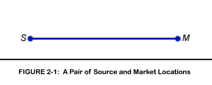
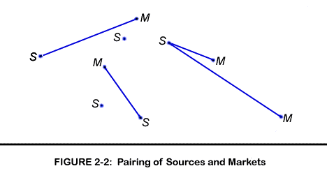
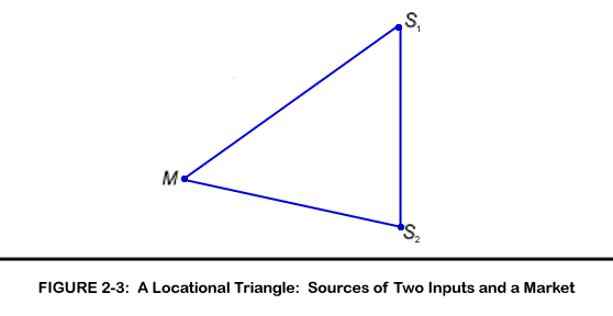
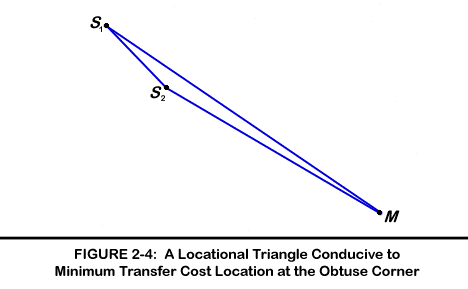
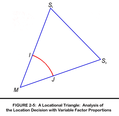
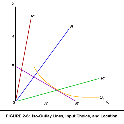
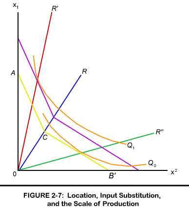
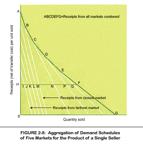